

三维分析直接展示小鼠桶皮层特异性血管分布和交叉桶分支
染色方法:
尼氏染色
标记方法:
Nissl染色
包埋方法:
树脂包埋
成像平台:
BioMapping 1000

cover
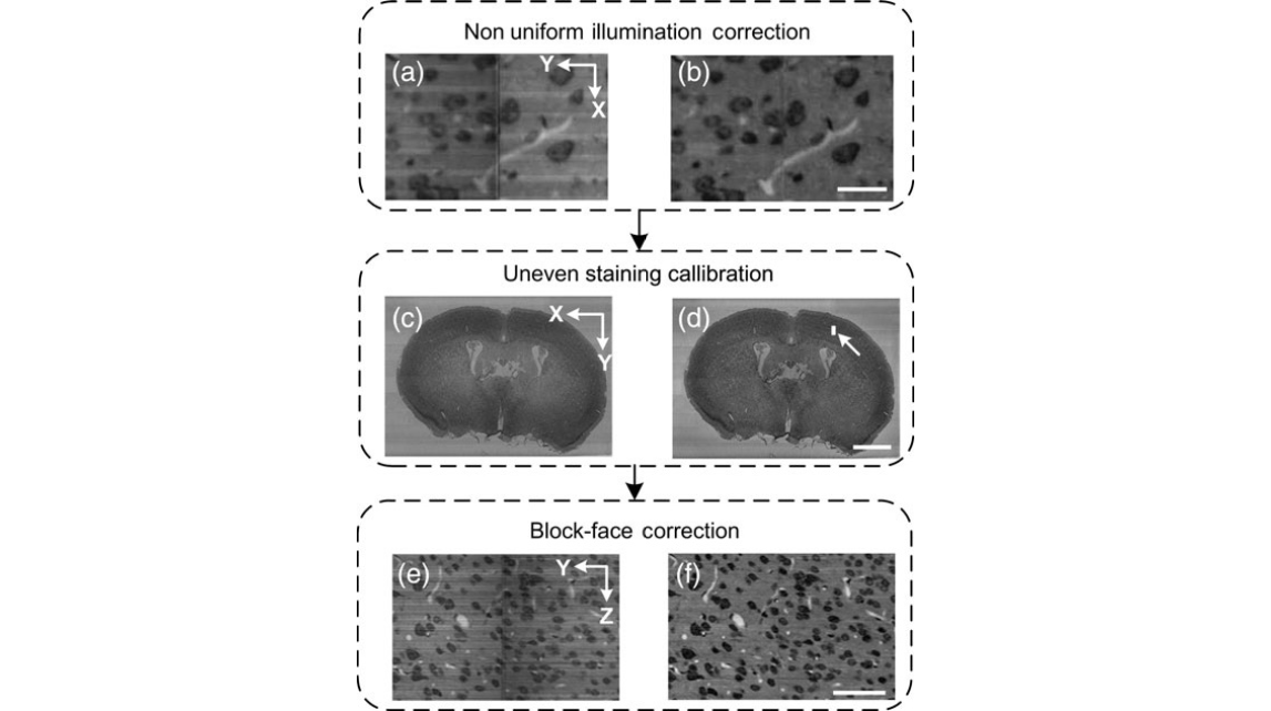
Figure 1. Image preprocessing pipeline. (a and b) The images before and after the nonuniform illumination correction show that the pixel intensity becomes uniform and the periodic noises are reduced. The morphology of both the cells and blood vessels that span the strip boundary was well maintained. The scale bar is 20 μm. (c and d) The coronal sections before and after the uneven staining calibration show that the coronal background intensity becomes uniform. The scale bar is 1 mm. (e and f) The background intensity among the coronal sections was adjusted to a constant after block-face correction. The scale bar is 50 μm. The intensity becomes uniform in 3D. (a, b, e, and f) are enlarged views of the region indicated by a white arrow in (d).
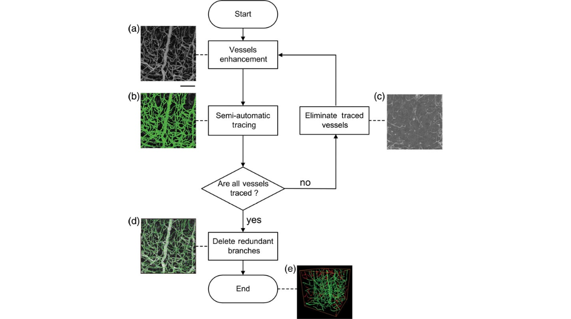
Figure 2. Schematic representation of the iterative vessel tracing strategy. (a) The maximum intensity projection shows a small interconnected vascular network that includes big and small vessels. The scale bar is 50 μm. (b) Most of the blood vessels were traced (green) using NeuronStudio by the first seed. (c) The traced blood vessels were eliminated using a customized MATLAB program, and the remaining vessels were visualized by a maximum intensity projection. (d) The tracing results were manually edited using Amira, and the redundant branches were deleted to enhance the precision. (e) 3D reconstruction of the final result. The red and green vessels represent the first tracing and the post-tracing result, respectively.

Figure 3. Simultaneous visualization of cells and blood vessels and the assessment of vectorization. (a) The preprocessed coronal image with a thickness of 1 μm shows the cross-sections of the cells and the vessels in the barrel field. (b) The minimum intensity projection of the image stack in (a) with a thickness of 30 μm. The cortical layers of I–VI were labeled according to cellular density aggregation. The light blue arrows indicate the dense aggregated cells of the barrel walls. (c) The maximum intensity projection of the image stack in (a) with a thickness of 200 μm. The position of some of the penetrating vessels matches that of the barrel walls that are visible in (b). (d) Qualitative assessment of the vessel tracing. The traced center lines were superimposed on the maximum projection of the preprocessed images with a thickness of 100 μm. (e) Quantitative assessment of the vessel tracing. The regions indicated by the red circuits are cross-sections of the tracing result. The light green arrow indicates a spurious vessel, and the yellow arrows indicate blood vessels that were not traced. All the scale bars in (a–e) are 100 μm.
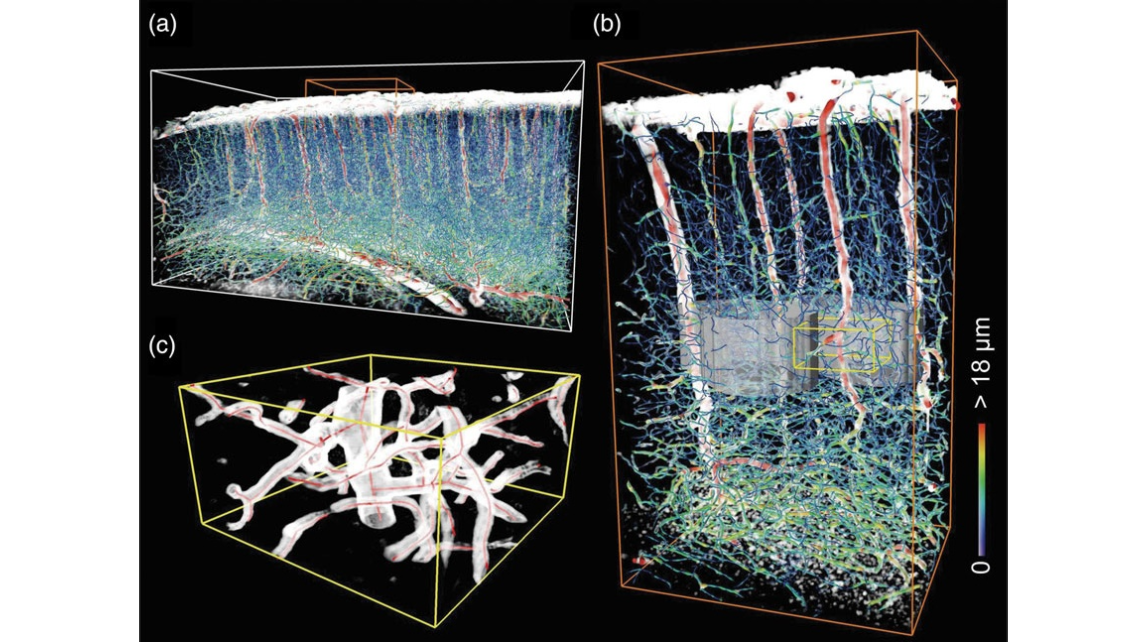
Figure 4. 3D reconstruction of the blood vessels in the barrel field. (a) The blood vessels were reconstructed by superimposing the vectorized result on a direct volume rendering. The size of the white bounding box is 1618 μm ×1082 μm ×870 μm. (b) An enlarged view of the orange box from (a) shows the vascular architecture near 2 barrels. The gray surfaces represent the barrel wall of C2 (left) and C3 (right). The size of the orange bounding box is 360 μm ×406 μm ×707 μm. The vascular diameter in (a and b) was color encoded by the color bar and was set to be half of the estimated value for clear comparison with the direct volume rendering. (c) An enlarged view of the yellow box from (b) shows the detailed local vascular architecture in layer IV. The traced center lines are represented by red curves in the direct volume rendering (white). The size of the yellow bounding box is 100 μm ×100 μm ×50 μm.

Figure 5. Vascular architecture among barrels in layer IV. (a) A direct volume rendering of layer IV in the barrel field with a thickness of 250 μm at a cortical depth of approximately 570 μm. The standard nomenclature for the barrels that consist of rows A–E and arcs 1–5 was identified according to the variation in the cellular density. The large penetrating vessels are represented by the red dots scattered in the interbarrel septa/barrel wall. The medial–lateral and anterior–posterior axes are indicated. (b) The maximum intensity projection of the image in (a) shows the vascular architecture in layer IV. The scale bar is 200 μm. (c) 3D reconstruction of penetrating vessels and barrels. The barrel walls are represented by gray surfaces. The yellow and red penetrating vessels have branches that extend across neighboring barrels, and the greenish vessels do not. The size of the white bounding box is 1082 μm ×1681 μm ×150 μm. (d) The penetrating vessel manually labeled red in c shows branches that extend across to neighboring barrels (C3 and C4) and a nonneighboring barrel (C5). Note that the trunk of this penetrating vessel locates in the interbarrel septa/barrel wall, and some neighboring barrels (D2 and D3) are not supplied or drained by this penetrating vessel.
Figure 6. Density profiles of the cells and blood vessels inside the barrel hollows. The cellular density profiles were grouped by arcs (a) and rows (b). The microvascular length density profiles were also grouped by arcs (c) and rows (d). The cortical layers of layer IV in (a–d) were identified based on the cellular density profile (a and b).
Video 1. Qualitative and quantitative assessment of cell localization. The cells are reconstructed by direct volume rendering (white). The manually labeled cells (red) and automatically detected cells (green) are represented by small spheres.
Video 2. 3D reconstruction of the blood vessels in the barrel field. The diameter of blood vessels is colour encoded. Note that the penetrating vessels localize outside the barrel walls. The diameter of traced blood vessels were set to half of the estimated diameter for clear comparison to the direct volume rendering.
cover
Figure 1. Image preprocessing pipeline. (a and b) The images before and after the nonuniform illumination correction show that the pixel intensity becomes uniform and the periodic noises are reduced. The morphology of both the cells and blood vessels that span the strip boundary was well maintained. The scale bar is 20 μm. (c and d) The coronal sections before and after the uneven staining calibration show that the coronal background intensity becomes uniform. The scale bar is 1 mm. (e and f) The background intensity among the coronal sections was adjusted to a constant after block-face correction. The scale bar is 50 μm. The intensity becomes uniform in 3D. (a, b, e, and f) are enlarged views of the region indicated by a white arrow in (d).
Figure 2. Schematic representation of the iterative vessel tracing strategy. (a) The maximum intensity projection shows a small interconnected vascular network that includes big and small vessels. The scale bar is 50 μm. (b) Most of the blood vessels were traced (green) using NeuronStudio by the first seed. (c) The traced blood vessels were eliminated using a customized MATLAB program, and the remaining vessels were visualized by a maximum intensity projection. (d) The tracing results were manually edited using Amira, and the redundant branches were deleted to enhance the precision. (e) 3D reconstruction of the final result. The red and green vessels represent the first tracing and the post-tracing result, respectively.
Figure 3. Simultaneous visualization of cells and blood vessels and the assessment of vectorization. (a) The preprocessed coronal image with a thickness of 1 μm shows the cross-sections of the cells and the vessels in the barrel field. (b) The minimum intensity projection of the image stack in (a) with a thickness of 30 μm. The cortical layers of I–VI were labeled according to cellular density aggregation. The light blue arrows indicate the dense aggregated cells of the barrel walls. (c) The maximum intensity projection of the image stack in (a) with a thickness of 200 μm. The position of some of the penetrating vessels matches that of the barrel walls that are visible in (b). (d) Qualitative assessment of the vessel tracing. The traced center lines were superimposed on the maximum projection of the preprocessed images with a thickness of 100 μm. (e) Quantitative assessment of the vessel tracing. The regions indicated by the red circuits are cross-sections of the tracing result. The light green arrow indicates a spurious vessel, and the yellow arrows indicate blood vessels that were not traced. All the scale bars in (a–e) are 100 μm.
Figure 4. 3D reconstruction of the blood vessels in the barrel field. (a) The blood vessels were reconstructed by superimposing the vectorized result on a direct volume rendering. The size of the white bounding box is 1618 μm ×1082 μm ×870 μm. (b) An enlarged view of the orange box from (a) shows the vascular architecture near 2 barrels. The gray surfaces represent the barrel wall of C2 (left) and C3 (right). The size of the orange bounding box is 360 μm ×406 μm ×707 μm. The vascular diameter in (a and b) was color encoded by the color bar and was set to be half of the estimated value for clear comparison with the direct volume rendering. (c) An enlarged view of the yellow box from (b) shows the detailed local vascular architecture in layer IV. The traced center lines are represented by red curves in the direct volume rendering (white). The size of the yellow bounding box is 100 μm ×100 μm ×50 μm.
Figure 5. Vascular architecture among barrels in layer IV. (a) A direct volume rendering of layer IV in the barrel field with a thickness of 250 μm at a cortical depth of approximately 570 μm. The standard nomenclature for the barrels that consist of rows A–E and arcs 1–5 was identified according to the variation in the cellular density. The large penetrating vessels are represented by the red dots scattered in the interbarrel septa/barrel wall. The medial–lateral and anterior–posterior axes are indicated. (b) The maximum intensity projection of the image in (a) shows the vascular architecture in layer IV. The scale bar is 200 μm. (c) 3D reconstruction of penetrating vessels and barrels. The barrel walls are represented by gray surfaces. The yellow and red penetrating vessels have branches that extend across neighboring barrels, and the greenish vessels do not. The size of the white bounding box is 1082 μm ×1681 μm ×150 μm. (d) The penetrating vessel manually labeled red in c shows branches that extend across to neighboring barrels (C3 and C4) and a nonneighboring barrel (C5). Note that the trunk of this penetrating vessel locates in the interbarrel septa/barrel wall, and some neighboring barrels (D2 and D3) are not supplied or drained by this penetrating vessel.
Figure 6. Density profiles of the cells and blood vessels inside the barrel hollows. The cellular density profiles were grouped by arcs (a) and rows (b). The microvascular length density profiles were also grouped by arcs (c) and rows (d). The cortical layers of layer IV in (a–d) were identified based on the cellular density profile (a and b).
Video 1. Qualitative and quantitative assessment of cell localization. The cells are reconstructed by direct volume rendering (white). The manually labeled cells (red) and automatically detected cells (green) are represented by small spheres.
Video 2. 3D reconstruction of the blood vessels in the barrel field. The diameter of blood vessels is colour encoded. Note that the penetrating vessels localize outside the barrel walls. The diameter of traced blood vessels were set to half of the estimated diameter for clear comparison to the direct volume rendering.
2016年1月26日,华中科技大学武汉光电国家研究中心骆清铭教授课题组,利用MOST技术,结合尼氏染色方法,同时显示单个细胞和血管,包括毛细血管,获得了覆盖整个小鼠桶状皮层的1微米分辨率3D 数据集。文章发表在《大脑皮层》杂志上。
参考文献
参考文献[1]:Wu J, Guo C, Chen S, et al. Direct 3D Analyses Reveal Barrel-Specific Vascular Distribution and Cross-Barrel Branching in the Mouse Barrel Cortex[J]. Cerebral Cortex, 2016, 26(1):23.