

小鼠大脑连接组高通量双色精细成像
染色方法:
PI实时复染
标记方法:
PI
包埋方法:
树脂包埋
成像平台:
BioMapping 3000
cover 1
cover 2

Figure 1 | Principle of BPS. (a) BPS Data acquisition overview. The resin-embedded sample moves between the SIM and the microtome. The SIM acquires three raw images to reconstruct an optical section and axially scans for Z-stack imaging over a certain range. The entire coronal section is imaged in a mosaic manner. (b) Schematic representation of the real-time cytoarchitecture staining. The dye molecules penetrate into the fresh resin-embedded sample surface and immediately combine with the nucleic acids inside the cell body. The soma is then visualized.
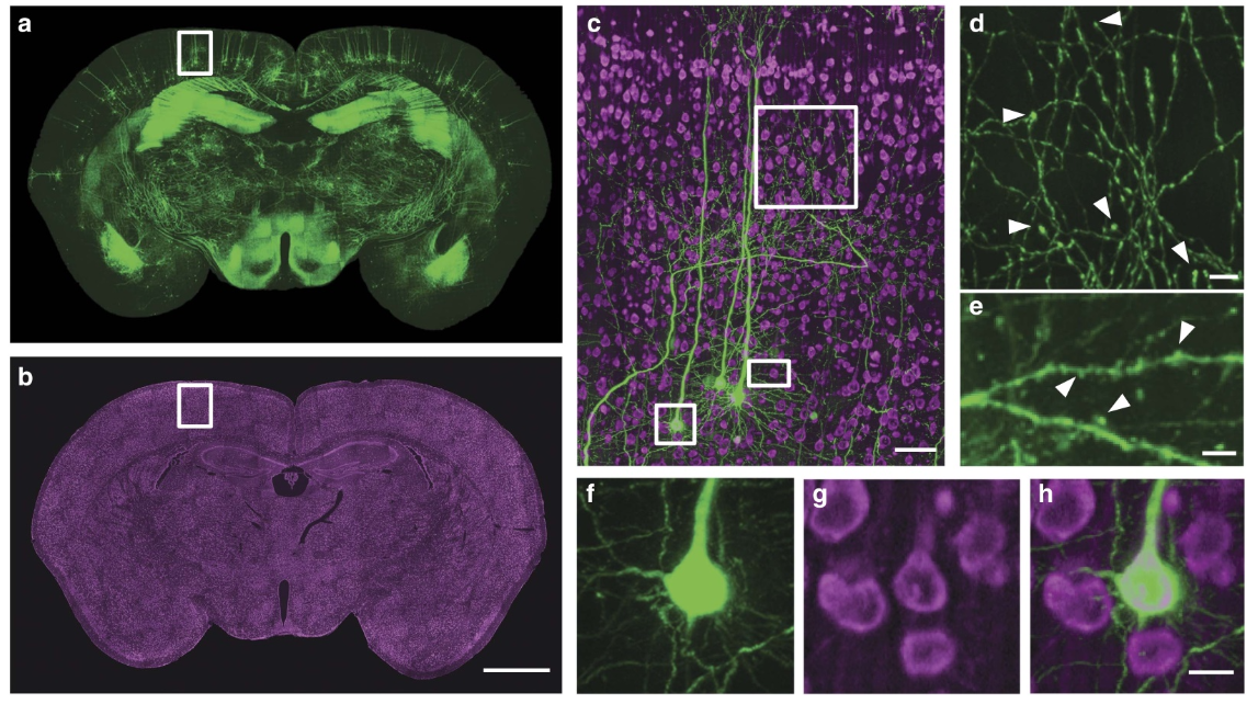
Figure 2 | Brain-wide dual-colour imaging of a Thy1-GFP M-line mouse brain. (a,b) Maximum intensity projections of the coronal sections. The projections were 400 (a) and 1 mm (b) thick. (c) Merged images indicated by the white boxes in a,b. (d) An enlarged view of the area indicated by the upper white square in c, demonstrating the visualization of axonal boutons, indicated using arrowheads. (e) An enlarged view of the area indicated by the white rectangle in c demonstrating visualization of dendritic spines, indicated using arrowheads. (f,g) Raw signals of the enlarged views of the area indicated by the lower white square in c. (h) Merged image, demonstrating accurate co-localization at single soma resolution using PI staining. (c,h) The projection thicknesses of GFP and PI were 400 mm and 1 mm, respectively. Scale bars, (a,b) 1 mm; (c) 50 mm; (d) 40 mm; (e) 5 mm; and (f–h) 10 mm.

Figure 3 | Continuous neural projections with high resolution. (a) 3D reconstruction of a GFP-labelled image block without preprocessing. The image block is selected from the same whole-brain data set of Fig. 2 and located in the thalamus. (b–d) Maximum intensity projections on transverse, sagittal and coronal sections, accordingly. Each projection depth is 400 mm. Scale bar, 50 mm.

Figure 4 | Localization and reconstruction of pyramidal neurons in the Thy1-GFP M-line mouse barrel field. (a) PI-channel volume rendering and the 220-mm-thick perspective projection of the barrel field of the right hemisphere, showing layer IV cytoarchitecture. Scale bar, 200 mm. (b) A reconstructed pyramidal neuron and associated cytoarchitecture reference. (left) Neuron and the local layer IV cytoarchitecture of the D3 and D4 columns (410 340 80 mm image stack). The apical dendrites of this neuron are located in the barrel hollow of D3. The blue arrow indicates the location where the neuron passes through the upper boundary of the image stack. (right) The cytoarchitecture from layer I to the corpus callosum surrounding the same neuron as shown on the left. The blue arrowheads indicate barrel walls. Image stack volume size: 760 850 150 mm. Scale bar, 100 mm. (c) 3D reconstruction of the barrel walls and 50 representative neurons located in the barrel field. The barrel walls were reconstructed according to PI-stained images and represented as gold loops (height: 80 mm). (d) The distribution of all long-range projection neurons among the 50 representative neurons. The thalamus, midbrain and medulla are the major projection regions. L, left; P, posterior; and V, ventral. (e) Ten reconstructed neurons (c) and corresponding barrel columns. The five neurons shown on the left are long-tufted pyramidal neurons, and the remaining five neurons are short-sparse neurons. The orange neuron located in D3 is the same neuron shown in b. Blue, green and orange colours represent neurons with axons extending the furthest to the striatum or thalamus, the midbrain and the pons or medulla, respectively. Pink denotes local projection neurons.
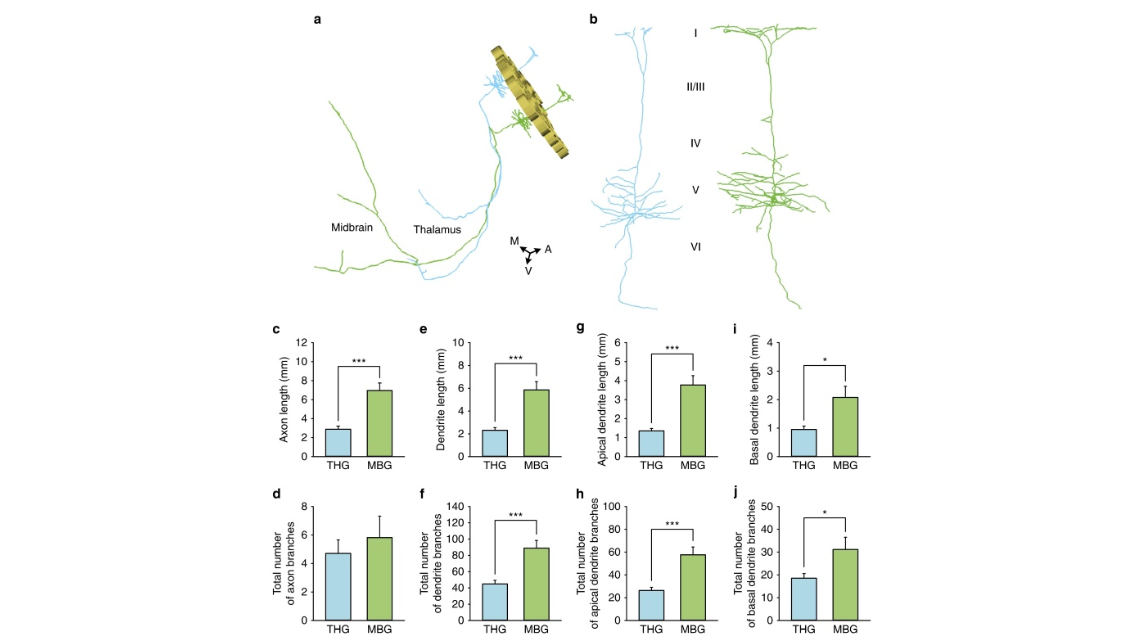
Figure 5 | Quantitative comparison of the fine morphology of neurons. (a) 3D reconstruction of the barrel walls and two representative long-range projection neurons located in the barrel cortex. The barrel walls were reconstructed according to PI-stained images and represented as gold loops (height: 80 mm). The blue neuron was localized to the D5 barrel column and projected to the thalamus. The green neuron was localized in the E2 barrel column and projected to the midbrain. A, anterior; M, middle; and V, ventral. (b) The enlarged views of the dendrites of the two neurons in (a) showing the distinct dendrite complexities of the projection neurons in the two groups. (c,d) Histograms of the axonal lengths (Po0.001) and branch numbers (P ¼ 0.520) of the long-range neurons, respectively. THG (n ¼ 15) and MBG (n ¼ 11) represent the neurons projecting to the thalamus and midbrain, respectively. (e,f) Histograms of the dendrite lengths (Po0.001) and branch numbers (Po0.001) of long-range neurons, respectively. (g,h) Histograms of the apical dendrite lengths (Po0.001) and branch numbers (Po0.001) of long-range neurons, respectively. (i,j) Histograms of the basal dendrite lengths (P ¼ 0.017) and branch numbers (P ¼ 0.045) of long-range neurons, respectively. We performed Student’s t-test on two groups by SPSS 22. Error bars were defined as s.e.m. Confidence level was set to 0.05 (P value). * represents P<0.05, and *** represents P<0.001.
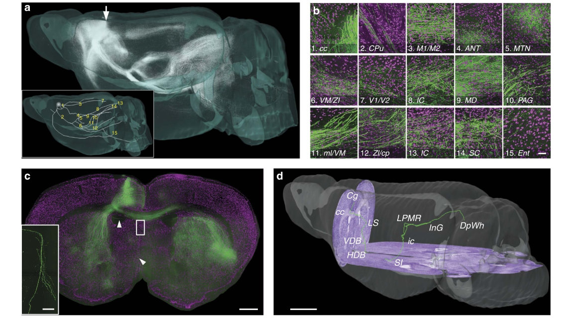
Figure 6 | Anterograde tracing and localization of brain-wide neural projections. (a) Anterograde projections of AAV-GFP-labelled Cg neurons in the entire brain. The inset shows the main pattern of the Cg projecting to the whole brain, and the 15 passing regions are indicated in the global observation at low resolution. The grey sphere indicates the injection site. (b) Merged local maximum intensity projections of the sagittal planes of the corresponding positions indicated in a. Passing regions: (b1) corpus callosum, (b2) caudate putamen, (b3) primary/secondary motor cortex, (b4) anteroventral thalamic nucleus and anterodorsal thalamic nucleus, (b5) anteromedial thalamic nucleus and paratenial thalamic nucleus, (b6) ventromedial thalamic nucleus, zona incerta dorsal part (ZID), zona incerta ventral part (ZIV), and reticular thalamic nucleus, (b7) primary/secondary visual cortex, (b8) inferior colliculus (ic), (b9) mediodorsal thalamic nucleus central part, mediodorsal thalamic nucleus dorsal part and mediodorsal thalamic nucleus lateral part, (b10) periaqueductal gray, (b11) medial lemniscus and ZID, (b12) ZID/ZIV and cerebral peduncle, (b13) ic, (b14) superior colliculus and (b15) entorhinal cortex. The size of each panel is 300 320 mm. Green represents the maximum intensity projections of GFP-labelled axons. The projection thickness shown in images 3, 5, 6, 9, 13 and 14 is 32 mm, and the projection thickness of the other images is 64 mm. Magenta represents PI-stained cells (2 mm thickness). (c) Projection pattern from Cg neurons on the coronal plane indicated with an arrow in (a). Green represents the maximum intensity projection of GFPlabelled projections (960 mm total thickness). Magenta represents PI-stained cells (2 mm thickness). The inset is an amplified image of the block shown in (c) containing sparse axons. (d) The reconstructed and localized axon indicated with arrowheads in (c). The cell body is located in the Cg region, and the axon connects to DpWh. Additionally, the axon bifurcates in the ic and LPMR brain regions. Purple represents the PI-counterstained cytoarchitecture background. Scale bar, 50 mm (b); 500 mm (c); 50 mm (the inset in c); and 100 mm (d).
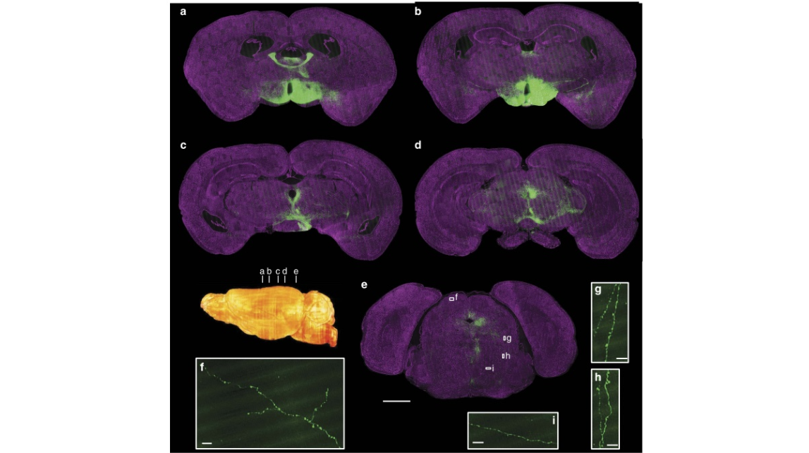
Figure 7 | Whole-brain imaging of GFP-labelled neurons in a SOM Cre-line mouse brain. (a–e) Maximum intensity projections of different coronal sections showing the projection patterns with cytoarchitectonic references. The inset shows locations of images shown in a–e. The projection thicknesses of GFP-signal were 60 mm (a,b), 120 mm (c) 200 mm (d) and 100 mm (e). Magenta represents PI-stained cells (2 mm thickness). (f–i) Representative raw images showing the fine structure, such as axon boutons, of the long-range projections shown in (e). Scale bar, 1 mm (a–e) and 15 mm (f–i).
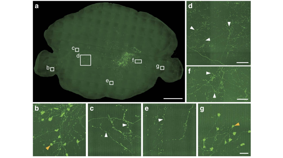
Figure 8 | Reconstruction of sparse-labelled brainstem neurons with long-range projections. (a) Maximum intensity projections of the coronal sections. The projection thickness was 900 mm. (b–g) Enlarged views of the single axon arbor and axon terminals of the neurons shown in a. The reconstructed boutons are indicated as white arrowheads. The large axon terminals were indicated as orange arrowheads. Scale bar, 1 mm (a); 100 mm (d); 50 mm (f); and 25 mm (b,c,e,g).
Movie 1: 3D reconstruction of the GFP-labeled image block shown in Fig. 3 without preprocessing.
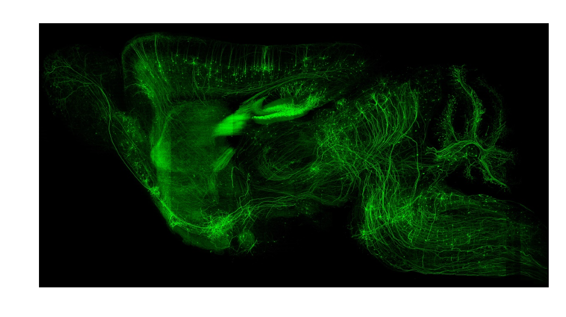
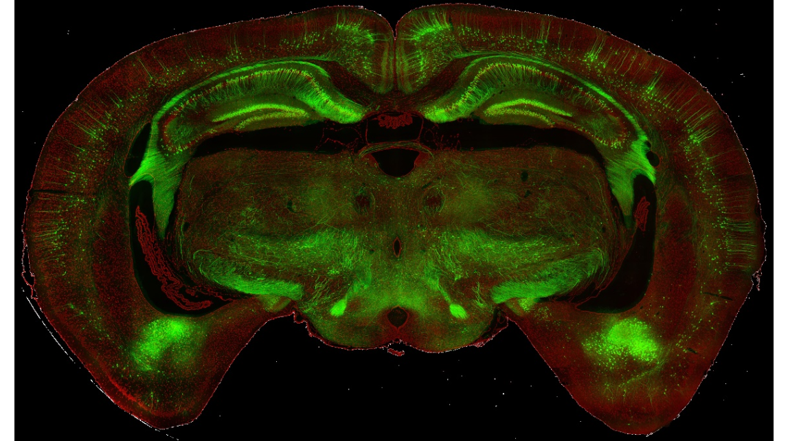
Movie 2: The image dataset of the whole Thy1-GFP M-line mouse brain obtained via WVT. In each section, red represents a 2-μm coronal image of PI-stained cells, and green represents a 200-μm coronal image of the maximum intensity projection of GFP-labeled neurons.
Movie 3: 3D reconstruction of a pyramidal neuron and the surrounding barrel cortex area of the Thy1-GFP M-line mouse brain. The Movie shows a pyramidal neuron and its location from layer I to the corpus callosum (corresponds to Fig. 4b). PI-stained cell bodies are in purple. The result shows that the soma of the pyramidal neuron is locating in layer V. The PI staining results clearly show layered structure of the barrel cortex and the precise locations of each cell body. The end of this Movie shows the reconstruction of the barrel walls. The size of data block is 760 × 850 × 150 μm3.
Movie 4: 2D consecutive slices showing the original images and axon tracing. The thickness of each slice is 16 μm, the size of display area is 220 × 160 μm, and the green signal is the tracing mark of the labeled axon on the current slice. The neuron is the green neuron in D5 in Fig. 4e.
Movie 5: Tracing of a pyramidal neuron in the Thy1-GFP M-line mouse brain overlaid with 3D image volume rendering. The 3D image volume is rendered from 12 blocks of 320 × 320 × 300 μm3 that the axon passed through at the voxel size of 0.32 × 0.32 × 2 μm. The tracing of the neuron is marked in red. There is 1-μm offset between tracing mark and volume data. Tracing the same pyramidal neuron as shown in Supplementary Movie 3 overlaid with the 3D image volume rendering.
Movie 6: Projections of pyramidal neurons in the barrel cortex of Thy1-GFP M-line brain. 3D view of Fig. 4d.
Movie 7: 3D reconstruction of the image dataset of the whole C57 mouse brain injected in Cg area with AAV-GFP and obtained via WVT. The same neuron as shown in Fig. 6. 3D volume rendering of the mouse brain is down-sampled at the voxel size of 2 × 2 × 2 μm due to the restriction of graphic card performance, and displayed with the manual outline segmentation of the whole mouse brain. Detailed volume views show the raw data in the thalamus, fibers in white and cell bodies in red. The size of the volume is 320 × 320 × 300 μm.
Movie 8: 3D volume rendering of the injection site. The same brain as shown in Supplementary Movie 7. The data size is 540 × 660 × 180 μm3 , and the location of the data corresponds to the block in Supplementary Figure 6a. The red spheres were detected by NeuronGPS to show the centers of each soma.
Movie 9: 2D consecutive slices showing the original images and AAV-labeled neuron tracing. The same neuron as shown in Fig. 6c.
Movie 10: 3D volume rendering of the AAV-labeled neuron. The same neuron as shown in Fig. 6c.
cover 1
cover 2
Figure 1 | Principle of BPS. (a) BPS Data acquisition overview. The resin-embedded sample moves between the SIM and the microtome. The SIM acquires three raw images to reconstruct an optical section and axially scans for Z-stack imaging over a certain range. The entire coronal section is imaged in a mosaic manner. (b) Schematic representation of the real-time cytoarchitecture staining. The dye molecules penetrate into the fresh resin-embedded sample surface and immediately combine with the nucleic acids inside the cell body. The soma is then visualized.
Figure 2 | Brain-wide dual-colour imaging of a Thy1-GFP M-line mouse brain. (a,b) Maximum intensity projections of the coronal sections. The projections were 400 (a) and 1 mm (b) thick. (c) Merged images indicated by the white boxes in a,b. (d) An enlarged view of the area indicated by the upper white square in c, demonstrating the visualization of axonal boutons, indicated using arrowheads. (e) An enlarged view of the area indicated by the white rectangle in c demonstrating visualization of dendritic spines, indicated using arrowheads. (f,g) Raw signals of the enlarged views of the area indicated by the lower white square in c. (h) Merged image, demonstrating accurate co-localization at single soma resolution using PI staining. (c,h) The projection thicknesses of GFP and PI were 400 mm and 1 mm, respectively. Scale bars, (a,b) 1 mm; (c) 50 mm; (d) 40 mm; (e) 5 mm; and (f–h) 10 mm.
Figure 3 | Continuous neural projections with high resolution. (a) 3D reconstruction of a GFP-labelled image block without preprocessing. The image block is selected from the same whole-brain data set of Fig. 2 and located in the thalamus. (b–d) Maximum intensity projections on transverse, sagittal and coronal sections, accordingly. Each projection depth is 400 mm. Scale bar, 50 mm.
Figure 4 | Localization and reconstruction of pyramidal neurons in the Thy1-GFP M-line mouse barrel field. (a) PI-channel volume rendering and the 220-mm-thick perspective projection of the barrel field of the right hemisphere, showing layer IV cytoarchitecture. Scale bar, 200 mm. (b) A reconstructed pyramidal neuron and associated cytoarchitecture reference. (left) Neuron and the local layer IV cytoarchitecture of the D3 and D4 columns (410 340 80 mm image stack). The apical dendrites of this neuron are located in the barrel hollow of D3. The blue arrow indicates the location where the neuron passes through the upper boundary of the image stack. (right) The cytoarchitecture from layer I to the corpus callosum surrounding the same neuron as shown on the left. The blue arrowheads indicate barrel walls. Image stack volume size: 760 850 150 mm. Scale bar, 100 mm. (c) 3D reconstruction of the barrel walls and 50 representative neurons located in the barrel field. The barrel walls were reconstructed according to PI-stained images and represented as gold loops (height: 80 mm). (d) The distribution of all long-range projection neurons among the 50 representative neurons. The thalamus, midbrain and medulla are the major projection regions. L, left; P, posterior; and V, ventral. (e) Ten reconstructed neurons (c) and corresponding barrel columns. The five neurons shown on the left are long-tufted pyramidal neurons, and the remaining five neurons are short-sparse neurons. The orange neuron located in D3 is the same neuron shown in b. Blue, green and orange colours represent neurons with axons extending the furthest to the striatum or thalamus, the midbrain and the pons or medulla, respectively. Pink denotes local projection neurons.
Figure 5 | Quantitative comparison of the fine morphology of neurons. (a) 3D reconstruction of the barrel walls and two representative long-range projection neurons located in the barrel cortex. The barrel walls were reconstructed according to PI-stained images and represented as gold loops (height: 80 mm). The blue neuron was localized to the D5 barrel column and projected to the thalamus. The green neuron was localized in the E2 barrel column and projected to the midbrain. A, anterior; M, middle; and V, ventral. (b) The enlarged views of the dendrites of the two neurons in (a) showing the distinct dendrite complexities of the projection neurons in the two groups. (c,d) Histograms of the axonal lengths (Po0.001) and branch numbers (P ¼ 0.520) of the long-range neurons, respectively. THG (n ¼ 15) and MBG (n ¼ 11) represent the neurons projecting to the thalamus and midbrain, respectively. (e,f) Histograms of the dendrite lengths (Po0.001) and branch numbers (Po0.001) of long-range neurons, respectively. (g,h) Histograms of the apical dendrite lengths (Po0.001) and branch numbers (Po0.001) of long-range neurons, respectively. (i,j) Histograms of the basal dendrite lengths (P ¼ 0.017) and branch numbers (P ¼ 0.045) of long-range neurons, respectively. We performed Student’s t-test on two groups by SPSS 22. Error bars were defined as s.e.m. Confidence level was set to 0.05 (P value). * represents P<0.05, and *** represents P<0.001.
Figure 6 | Anterograde tracing and localization of brain-wide neural projections. (a) Anterograde projections of AAV-GFP-labelled Cg neurons in the entire brain. The inset shows the main pattern of the Cg projecting to the whole brain, and the 15 passing regions are indicated in the global observation at low resolution. The grey sphere indicates the injection site. (b) Merged local maximum intensity projections of the sagittal planes of the corresponding positions indicated in a. Passing regions: (b1) corpus callosum, (b2) caudate putamen, (b3) primary/secondary motor cortex, (b4) anteroventral thalamic nucleus and anterodorsal thalamic nucleus, (b5) anteromedial thalamic nucleus and paratenial thalamic nucleus, (b6) ventromedial thalamic nucleus, zona incerta dorsal part (ZID), zona incerta ventral part (ZIV), and reticular thalamic nucleus, (b7) primary/secondary visual cortex, (b8) inferior colliculus (ic), (b9) mediodorsal thalamic nucleus central part, mediodorsal thalamic nucleus dorsal part and mediodorsal thalamic nucleus lateral part, (b10) periaqueductal gray, (b11) medial lemniscus and ZID, (b12) ZID/ZIV and cerebral peduncle, (b13) ic, (b14) superior colliculus and (b15) entorhinal cortex. The size of each panel is 300 320 mm. Green represents the maximum intensity projections of GFP-labelled axons. The projection thickness shown in images 3, 5, 6, 9, 13 and 14 is 32 mm, and the projection thickness of the other images is 64 mm. Magenta represents PI-stained cells (2 mm thickness). (c) Projection pattern from Cg neurons on the coronal plane indicated with an arrow in (a). Green represents the maximum intensity projection of GFPlabelled projections (960 mm total thickness). Magenta represents PI-stained cells (2 mm thickness). The inset is an amplified image of the block shown in (c) containing sparse axons. (d) The reconstructed and localized axon indicated with arrowheads in (c). The cell body is located in the Cg region, and the axon connects to DpWh. Additionally, the axon bifurcates in the ic and LPMR brain regions. Purple represents the PI-counterstained cytoarchitecture background. Scale bar, 50 mm (b); 500 mm (c); 50 mm (the inset in c); and 100 mm (d).
Figure 7 | Whole-brain imaging of GFP-labelled neurons in a SOM Cre-line mouse brain. (a–e) Maximum intensity projections of different coronal sections showing the projection patterns with cytoarchitectonic references. The inset shows locations of images shown in a–e. The projection thicknesses of GFP-signal were 60 mm (a,b), 120 mm (c) 200 mm (d) and 100 mm (e). Magenta represents PI-stained cells (2 mm thickness). (f–i) Representative raw images showing the fine structure, such as axon boutons, of the long-range projections shown in (e). Scale bar, 1 mm (a–e) and 15 mm (f–i).
Figure 8 | Reconstruction of sparse-labelled brainstem neurons with long-range projections. (a) Maximum intensity projections of the coronal sections. The projection thickness was 900 mm. (b–g) Enlarged views of the single axon arbor and axon terminals of the neurons shown in a. The reconstructed boutons are indicated as white arrowheads. The large axon terminals were indicated as orange arrowheads. Scale bar, 1 mm (a); 100 mm (d); 50 mm (f); and 25 mm (b,c,e,g).
Movie 1: 3D reconstruction of the GFP-labeled image block shown in Fig. 3 without preprocessing.
Movie 2: The image dataset of the whole Thy1-GFP M-line mouse brain obtained via WVT. In each section, red represents a 2-μm coronal image of PI-stained cells, and green represents a 200-μm coronal image of the maximum intensity projection of GFP-labeled neurons.
Movie 3: 3D reconstruction of a pyramidal neuron and the surrounding barrel cortex area of the Thy1-GFP M-line mouse brain. The Movie shows a pyramidal neuron and its location from layer I to the corpus callosum (corresponds to Fig. 4b). PI-stained cell bodies are in purple. The result shows that the soma of the pyramidal neuron is locating in layer V. The PI staining results clearly show layered structure of the barrel cortex and the precise locations of each cell body. The end of this Movie shows the reconstruction of the barrel walls. The size of data block is 760 × 850 × 150 μm3.
Movie 4: 2D consecutive slices showing the original images and axon tracing. The thickness of each slice is 16 μm, the size of display area is 220 × 160 μm, and the green signal is the tracing mark of the labeled axon on the current slice. The neuron is the green neuron in D5 in Fig. 4e.
Movie 5: Tracing of a pyramidal neuron in the Thy1-GFP M-line mouse brain overlaid with 3D image volume rendering. The 3D image volume is rendered from 12 blocks of 320 × 320 × 300 μm3 that the axon passed through at the voxel size of 0.32 × 0.32 × 2 μm. The tracing of the neuron is marked in red. There is 1-μm offset between tracing mark and volume data. Tracing the same pyramidal neuron as shown in Supplementary Movie 3 overlaid with the 3D image volume rendering.
Movie 6: Projections of pyramidal neurons in the barrel cortex of Thy1-GFP M-line brain. 3D view of Fig. 4d.
Movie 7: 3D reconstruction of the image dataset of the whole C57 mouse brain injected in Cg area with AAV-GFP and obtained via WVT. The same neuron as shown in Fig. 6. 3D volume rendering of the mouse brain is down-sampled at the voxel size of 2 × 2 × 2 μm due to the restriction of graphic card performance, and displayed with the manual outline segmentation of the whole mouse brain. Detailed volume views show the raw data in the thalamus, fibers in white and cell bodies in red. The size of the volume is 320 × 320 × 300 μm.
Movie 8: 3D volume rendering of the injection site. The same brain as shown in Supplementary Movie 7. The data size is 540 × 660 × 180 μm3 , and the location of the data corresponds to the block in Supplementary Figure 6a. The red spheres were detected by NeuronGPS to show the centers of each soma.
Movie 9: 2D consecutive slices showing the original images and AAV-labeled neuron tracing. The same neuron as shown in Fig. 6c.
Movie 10: 3D volume rendering of the AAV-labeled neuron. The same neuron as shown in Fig. 6c.
2016年7月4日,华中科技大学武汉光电国家研究中心龚辉老师课题组使用fMOST技术首次展示了当前世界最精细的荧光小鼠全脑数据集,文章发表在《自然-通讯》杂志。
参考文献
参考文献[1]:Gong H, Xu D, Yuan J, Li X, Guo C, Peng J, Li Y, Schwarz LA, Li A, Hu B, Xiong B, Sun Q, Zhang Y, Liu J, Zhong Q, Xu T, Zeng S, Luo Q. High-throughput dual-colour precision imaging for brain-wide connectome with cytoarchitectonic landmarks at the cellular level. Nat Commun. (2016);7:12142.