

皮质轴突细胞神经元的全脑展示
染色方法:
病毒示踪标记
标记方法:
GFP、 YFP、 RFP
包埋方法:
树脂包埋
成像平台:
BioMapping 3000

cover

Figure 1. Schematic of the gSNA Platform Applied to the Mouse Brain (A) Pipeline and components of genetic single neuron anatomy (gSNA). (B) Left: scheme of genetic and viral strategy for the labeling of axo-axonic cells (AACs). A transient CreER activity in MGE progenitors is converted to a constitutive Flp activity in mature AACs. Flp-dependent AAVs injected in specific cortical areas enables sparse and robust AAC labeling. (C) fMOST high-resolution whole-brain imaging. Two-color imaging for the acquisition of GFP (green) channel and PI (propidium iodide, red) channel signals. PI stains brain cytoarchitecture in real time, and therefore provides each dataset with a self-registered atlas. A 488-nm wavelength laser was used for the excitation of both GFP and PI signals. Whole-brain coronal image stacks were obtained by sectioning (with a diamond knife) and imaging cycles at 1-μm z steps, guided by a motorized precision XYZ stage.
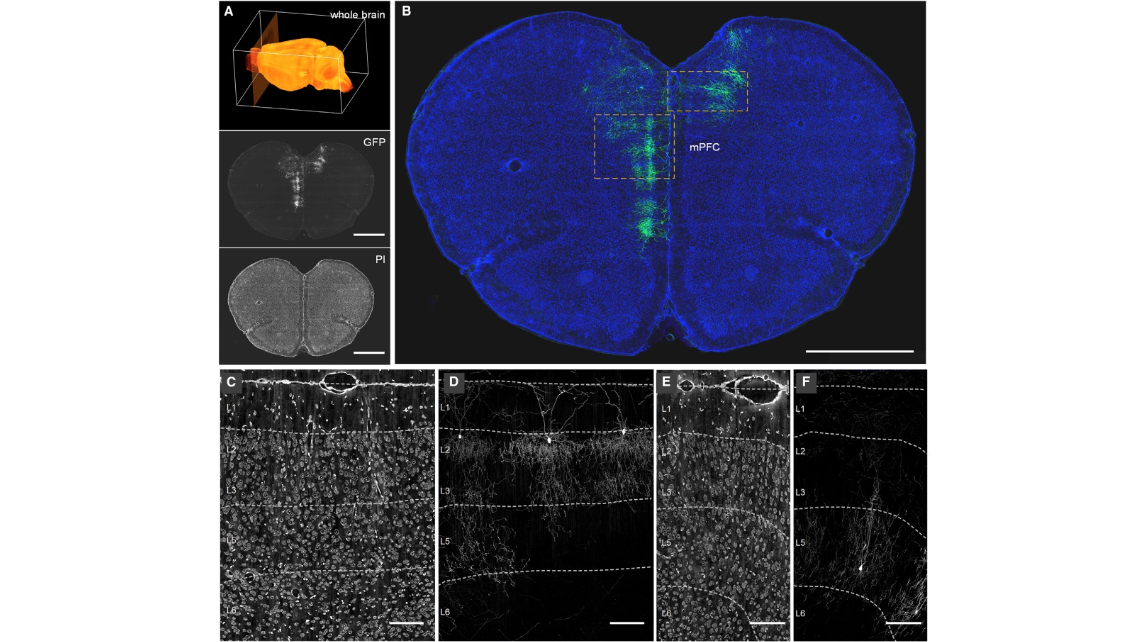
Figure 2. Areal and Laminar Distribution of AACs Revealed from Whole-Brain fMOST Dataset (A) A schematic of whole-brain coronal dataset collection (top) with an example of GFP channel (center) and PI channel (bottom) images. Scale bars: 1,000 μm. (B) An example of the distribution of sparsely labeled AACs in mPFC. Green: AAC morphology, 100-μm max-intensity projection. Blue: cytoarchitecture revealed by PI, 5-μm max-intensity projection. Scale bar: 1,000 μm. (C and D) Laminar distribution of L2 AACs in mPFC. Enlargement of PI channel (C) and GFP channel (D) images from the left box in (B). (E and F) Laminar distribution of L5 AACs in mPFC. Enlargement of PI channel (E) and GFP channel (F) images from the right box in (B). Dashed lines in (C)–(F) indicate the layer boundaries. Cortical layers were discriminated based on cell body distributions in PI channel according to the Allen Mouse Brain Reference Atlas (http://portal.brain-map.org/). Scale bars in (E) and (F): 100 μm.
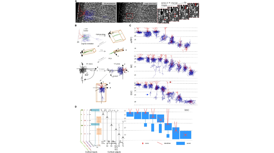
Figure 3. Single AAC Reconstructions in Cerebral Cortex (A) A representative AAC reconstruction and its co-registered PI channel images. Left: overlay of the reconstructed cell with its PI channel image (10-μm max intensity projection) with the original orientation. Cytoarchitecture information shows the cortical laminar organization (more details in STAR Methods). Scale bar: 50 μm. Middle: single slice of PI channel. Right: enlarged image series from the boxed area in middle panel. Arrows indicate a pyramidal neuron main dendrite extending from cell body. Scale bar: 15 μm. (B) Rotation and alignment procedures based on reconstructed pyramidal dendrites (green). Randomly selected pyramidal dendrites near the AAC cell body were reconstructed in Neurolucida360. The vertical axis of the local cortical column was calculated by performing principal-component analysis (PCA) on the centered dendritic reconstructions. AAC reconstruction was then re-aligned in the coronal plane (XY plane) and sagittal plane (YZ plane) around the cell body based on the identified cortical column orientation. (C) Representative AAC single-cell reconstructions in mPFC, MC, and SSC. Cortical layers in each area were indicated by dashed lines. Black: soma body. Red: dendrites. Blue: axons. The orientation of each reconstruction was re-adjusted according to the local cortical vertical axis (see more details in STAR Methods). Representative translaminar axonal and dendritic arbors in the SSC are indicated by blue and red arrows, respectively. (D) Left: scheme of the laminar arrangement of the input and output streams of SSC, in part rooted in the laminar organization of pyramidal neuron types with distinct projection targets. Right: a schematic of representative AACs in the SSC with characteristic laminar dendritic and axonal distribution patterns. Str, striatum; Bsm, brainstem; Scd, spinal cord; SCs, superior colliculus; Pom, posterior complex of thalamus; VPM, ventral posteromedial nucleus of the thalamus; Th, thalamus; ipsi, ipsilateral; contra, contralateral.
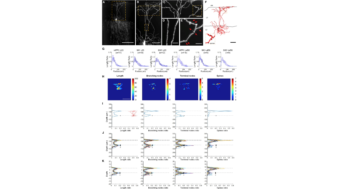
Figure 4. Characteristics of L2 AAC Dendrites (A) A representative L2 AAC in mPFC. 100-μm max intensity projection. Scale bar: 100 μm. (B) Dendrites of L2 AAC. Image was enlarged from the box in (A). Scale bar: 50 μm. (C and D) Apical (C) and main dendrites (D) were enlarged from boxes in (B). Scale bars: 30 μm (C) and 5 μm (D). (E) Spines (arrows) on the apical dendrites were enlarged from the box in (C). Scale bar: 5 μm. (F) Complete reconstruction of dendrites (red) and spines (black). The same cell shown in (A) and (B). Inset: enlarged from the box. Black circle: cell body. Gray lines: pia and L1/2 border. Scale bar: 50 μm. (G) Horizontal dendritic arbor distributions of up-layer (L2 and L3) and deep-layer (L4, L5 and L6) AACs in mPFC, MC, and SSC. Data are mean ± SD. (H) An example of heatmaps showing the density distribution patterns of a L2 AAC dendritic arbor length (left), branching nodes (middle left), terminal nodes (middle right), and spines (right). Scale bar: 200 μm. (I) Single-cell density plots of L2 AAC dendrites (same as in H) along the cortical depth. (J) Density plots of dendrites from 11 L2 AACs in mPFC. Different colors indicate different cells. (K) Normalized density plots of (J) based on pia and L1/2 border positions (see more details in STAR Methods). Black circles in (I)–(K) indicate AAC soma positions in the coordinate. Dashed lines correspond to the place of pia (top) and L1/2 border (bottom). Dark black curves in (J) and (K) are averages of all the cells. Density value was presented by ratio.

Figure 5. Morphology and Distribution Patterns of AAC Axons in the Neocortex (A) A representative images of two examples of nearby intra- (left) and cross- (right) L2 AACs in mPFC. Insets are enlarged images from boxed regions showing the main axon extending from the soma (1; arrow), characteristic axon cartridge clusters, and individual boutons from different regions of the axon arbor (2, 3, and 4). Image is a projection of 100-μm image stack. Scale bars: 100 μm (low-mag image) and 10 μm (insets). (B) A representative image containing nearby L2, L4, and L5 AACs in SSC. Enlarged L4 and L5 AACs were from the boxes in the left panel. Scale bars: 100 μm (left) and 10 μm (right). Dashed lines in (A) and (B) indicate cortical layers. (C) Horizontal axon arbor distributions of up-layer (L2 and L3) and deep-layer (L4, L5 and L6) AACs in mPFC, MC, and SSC. Data are mean ± SD. (D) Length density analysis of axons and dendrites from all the AACs shown in (A) and (B). Left: projection of reconstructions (dendrites in red; axons in blue). Middle: heatmap of length density distribution of dendrites (middle left) and axons (middle right). Right: length density plots of AAC dendrites and axons along cortical depth (y axis). Dashed lines indicate layer boundaries. Insets in rows 3 and 4 highlight axon branches in deep layers. (E) An example of axon bouton reconstruction of L2 AAC in mPFC. Inset: magnified view of the boxed region. (F) Axon cartridges that innervate PyN AIS can point upward, downward, or split from the middle. (G and H) The numbers of synaptic boutons correlate with axon length quantified by absolute value (G) or ratio (H).

Figure 6. Hierarchical Clustering of AACs Based on Cortical Laminar Density Distribution of Axons and Dendrites (A) Dendrogram of hierarchically clustered AACs (n = 53). KL divergences (Kullback-Leibler divergence) of normalized arbor distribution functions along cortical depth were taken as the distance metric, and furthest distance was taken as the linkage rule. See more details in STAR Methods and Figure S6 for the normalization procedures. Dashed lines correspond to the cutoff linkages of the identified eight cell clusters. Inset: silhouette analysis of the eight AAC clusters. (B) 3D scattering plots of the eight AAC clusters from (A) based on three principal components. (C) Axon (blue) and dendrite (red) length density distribution profiles of the eight AAC clusters. Dashed lines: cortical layer boundaries. Black circles: soma body positions. Bold lines: average of all the neurons in each cluster. Note that cell #38 in cluster 5 has apical dendrites (arrow) reading L1, a defining feature of cluster 6, but its lack of L3 axon branches (as it is located in SSC with a prominent L4) likely assigned it to cluster 5. (D–G) Clique analysis for the identification of robust AAC clusters. Clique analysis was conducted based on hierarchical clustering with five different metrics on AAC axons: three persistent-homology-based metrics, using three different ways of measuring distance from the soma, as scalar descriptor functions defined on the neuronal processes: Euclidean, geodesic, and depth from cortical surface (“y axis”), and the length density and L-measure metrics (Scorcioni et al., 2008) defined in the text (D and E). Laplacian eigenmap embedding of hierarchical clustering for the y axis-based metric (D) and other descriptors (Figure S7A–S7E). The selection of “K” was based on silhouette analysis. Silhouette plot for K = 4 with y axis as the input metric; thickness denotes sizes of clusters; red dotted line denotes average silhouette score; larger score means better clustering (E). The relations between the five metrics were quantified by similar index (SI) and adjusted Rand index (F). Three robust AAC clusters were identified based on the clique analysis (G). The full listing of the three cliques are shown in Figure S7F.
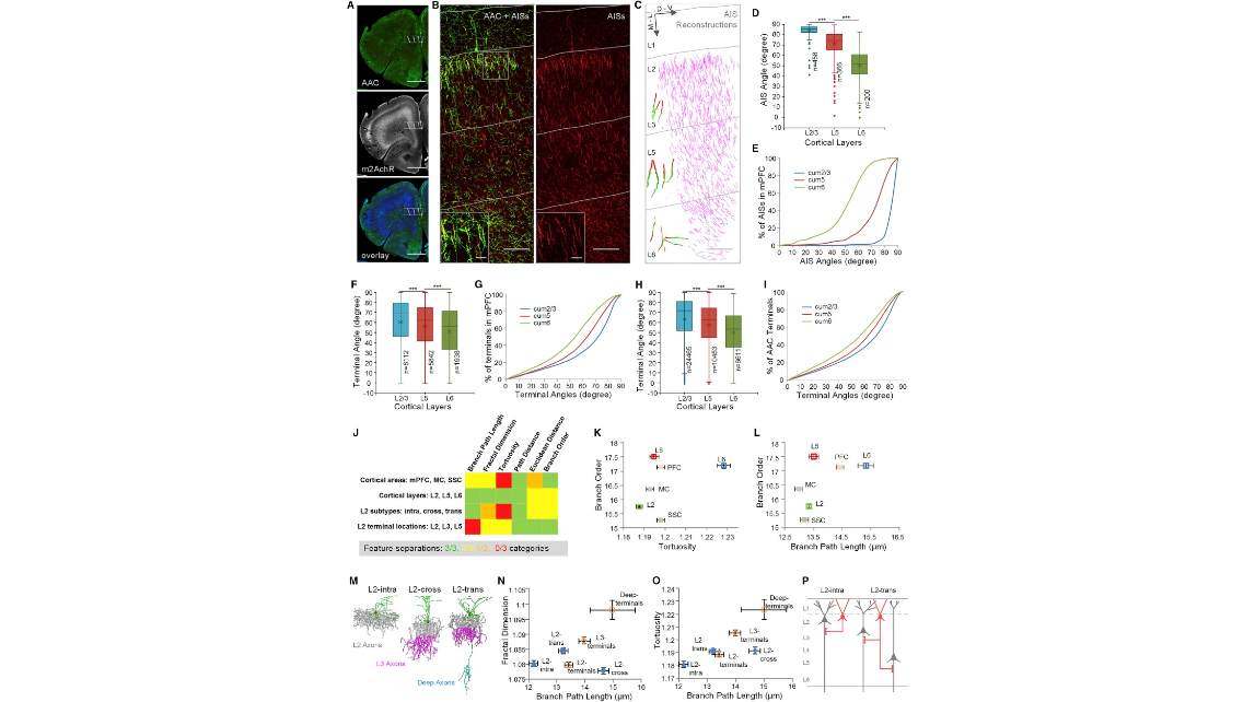
Figure 7. AAC Subtypes Revealed by Axon Terminal Characteristics That Correlate with AIS (A) Distributions of AACs in mPFC (50 μm thick). AACs were labeled by the crossing of Nkx2.1-CreER mouse and Ai14 (LSL-tdTomato) mouse with low dose of TM induction at E18.5. Top: AACs (green) shown by the immunostaining of tdTomato. Center: cortical layers shown by the immunostaining of m2AchR. Bottom: color merged. Scale bar: 1,000 μm. (B) AIS distributions in PrL (prelimbic cortex). Images were captured from the box in (A). Left: overlay image of AAC (green) and AIS (red). Right: immunostaining of AISs with Ankyrin-G. Insets: enlarged images. Gray lines indicate layer boundaries. Scale bars: 100 μm (low-mag) and 20 μm (insets). (C) AIS reconstructions (purple). Insets: representative reconstructions of presynaptic AAC cartridge and postsynaptic PyN AIS pairs in L2/3, L5, and L6. Green: cartridges. Red: AISs. Scale bar: 100 μm. (D and E) Distribution differences of AIS angles among cortical layers in mPFC (∗∗∗p < 0.0001, 95% confidence level, Kruskal-Wallis test followed by Dunn’s multiple-comparisons test). Plots indicate median (full horizontal bar), mean (×), quartiles, and range. AIS data (D) and cumulative plots (E) are from the reconstructions in (C). (F and G) The corresponding distribution differences of AAC axon terminal angles in mPFC (∗∗∗p < 0.0001, 95% confidence level, Kruskal-Wallis test followed by Dunn’s multiple-comparisons test). Plots indicate median (full horizontal bar), mean (×), quartiles, and range. Axon terminal data (F) and cumulative plots (G) are extracted from all our AAC reconstructions in mPFC (Figure S2A). (H and I) Averaged distribution differences of AAC axon terminal angles across mPFC, MC, and SSC (∗∗∗p < 0.0001, 95% confidence level, Kruskal-Wallis test followed by Dunn’s multiple-comparisons test). Plots indicate median (full horizontal bar), mean (×), quartiles, and range. Axon terminal data (H) and cumulative plots (I) are extracted from all our AAC reconstructions (Figure S2A). (J) Summary of axon terminal geometric features that separate AAC categories (cortical areas and cortical layers refer to somatic location). Green: statistically significant differences between all three pairs compared. Yellow: statistically significant differences between two of three pairs compared. Orange: statistically significant differences between one of three pairs compared. Red: no statistically significant differences. (K and L) Areal and laminar categories of AACs separated by axon terminal geometric parameters. Parameter pairs of branch order and (K) branch tortuosity or (L) branch path length are shown. Data are mean ± SEM. (M) Reconstructions of representative L2 AAC subtypes (L2-intra, L2-cross, and L2-trans). (N and O) Axon terminal geometric parameters separate L2 AAC subtypes. Parameter pairs of branch path length and (N) branch fractal dimension or (O) branch tortuosity are show. Data are mean ± SEM. (P) Schematic of inferred L2 AAC connectivity with PyNs.
Video S1. dfMOST Imaging of Viral-Labeled AACs at Single-Axon Resolution, Related to Figure 1. 100 μm max intensity projection of original GFP channel images without any imaging processing.
Video S2. Nearby L2-Intra and L2-Cross AACs in mPFC, Related to Figure 3
Video S3. Reconstructions of Nearby L2-Intra and L2-Cross AACs in mPFC, Related to Figure 3
Video S4. Reconstructions of Nearby L3 and L5-Intra AACs in MC, Related to Figure 3
Video S5. A L5a (L5-cross) AAC in mPFC, Related to Figure 3
Video S6. Nearby L4 and L6a (L5/L6 border) AAC in SSC, Related to Figure 3
cover
Figure 1. Schematic of the gSNA Platform Applied to the Mouse Brain (A) Pipeline and components of genetic single neuron anatomy (gSNA). (B) Left: scheme of genetic and viral strategy for the labeling of axo-axonic cells (AACs). A transient CreER activity in MGE progenitors is converted to a constitutive Flp activity in mature AACs. Flp-dependent AAVs injected in specific cortical areas enables sparse and robust AAC labeling. (C) fMOST high-resolution whole-brain imaging. Two-color imaging for the acquisition of GFP (green) channel and PI (propidium iodide, red) channel signals. PI stains brain cytoarchitecture in real time, and therefore provides each dataset with a self-registered atlas. A 488-nm wavelength laser was used for the excitation of both GFP and PI signals. Whole-brain coronal image stacks were obtained by sectioning (with a diamond knife) and imaging cycles at 1-μm z steps, guided by a motorized precision XYZ stage.
Figure 2. Areal and Laminar Distribution of AACs Revealed from Whole-Brain fMOST Dataset (A) A schematic of whole-brain coronal dataset collection (top) with an example of GFP channel (center) and PI channel (bottom) images. Scale bars: 1,000 μm. (B) An example of the distribution of sparsely labeled AACs in mPFC. Green: AAC morphology, 100-μm max-intensity projection. Blue: cytoarchitecture revealed by PI, 5-μm max-intensity projection. Scale bar: 1,000 μm. (C and D) Laminar distribution of L2 AACs in mPFC. Enlargement of PI channel (C) and GFP channel (D) images from the left box in (B). (E and F) Laminar distribution of L5 AACs in mPFC. Enlargement of PI channel (E) and GFP channel (F) images from the right box in (B). Dashed lines in (C)–(F) indicate the layer boundaries. Cortical layers were discriminated based on cell body distributions in PI channel according to the Allen Mouse Brain Reference Atlas (http://portal.brain-map.org/). Scale bars in (E) and (F): 100 μm.
Figure 3. Single AAC Reconstructions in Cerebral Cortex (A) A representative AAC reconstruction and its co-registered PI channel images. Left: overlay of the reconstructed cell with its PI channel image (10-μm max intensity projection) with the original orientation. Cytoarchitecture information shows the cortical laminar organization (more details in STAR Methods). Scale bar: 50 μm. Middle: single slice of PI channel. Right: enlarged image series from the boxed area in middle panel. Arrows indicate a pyramidal neuron main dendrite extending from cell body. Scale bar: 15 μm. (B) Rotation and alignment procedures based on reconstructed pyramidal dendrites (green). Randomly selected pyramidal dendrites near the AAC cell body were reconstructed in Neurolucida360. The vertical axis of the local cortical column was calculated by performing principal-component analysis (PCA) on the centered dendritic reconstructions. AAC reconstruction was then re-aligned in the coronal plane (XY plane) and sagittal plane (YZ plane) around the cell body based on the identified cortical column orientation. (C) Representative AAC single-cell reconstructions in mPFC, MC, and SSC. Cortical layers in each area were indicated by dashed lines. Black: soma body. Red: dendrites. Blue: axons. The orientation of each reconstruction was re-adjusted according to the local cortical vertical axis (see more details in STAR Methods). Representative translaminar axonal and dendritic arbors in the SSC are indicated by blue and red arrows, respectively. (D) Left: scheme of the laminar arrangement of the input and output streams of SSC, in part rooted in the laminar organization of pyramidal neuron types with distinct projection targets. Right: a schematic of representative AACs in the SSC with characteristic laminar dendritic and axonal distribution patterns. Str, striatum; Bsm, brainstem; Scd, spinal cord; SCs, superior colliculus; Pom, posterior complex of thalamus; VPM, ventral posteromedial nucleus of the thalamus; Th, thalamus; ipsi, ipsilateral; contra, contralateral.
Figure 4. Characteristics of L2 AAC Dendrites (A) A representative L2 AAC in mPFC. 100-μm max intensity projection. Scale bar: 100 μm. (B) Dendrites of L2 AAC. Image was enlarged from the box in (A). Scale bar: 50 μm. (C and D) Apical (C) and main dendrites (D) were enlarged from boxes in (B). Scale bars: 30 μm (C) and 5 μm (D). (E) Spines (arrows) on the apical dendrites were enlarged from the box in (C). Scale bar: 5 μm. (F) Complete reconstruction of dendrites (red) and spines (black). The same cell shown in (A) and (B). Inset: enlarged from the box. Black circle: cell body. Gray lines: pia and L1/2 border. Scale bar: 50 μm. (G) Horizontal dendritic arbor distributions of up-layer (L2 and L3) and deep-layer (L4, L5 and L6) AACs in mPFC, MC, and SSC. Data are mean ± SD. (H) An example of heatmaps showing the density distribution patterns of a L2 AAC dendritic arbor length (left), branching nodes (middle left), terminal nodes (middle right), and spines (right). Scale bar: 200 μm. (I) Single-cell density plots of L2 AAC dendrites (same as in H) along the cortical depth. (J) Density plots of dendrites from 11 L2 AACs in mPFC. Different colors indicate different cells. (K) Normalized density plots of (J) based on pia and L1/2 border positions (see more details in STAR Methods). Black circles in (I)–(K) indicate AAC soma positions in the coordinate. Dashed lines correspond to the place of pia (top) and L1/2 border (bottom). Dark black curves in (J) and (K) are averages of all the cells. Density value was presented by ratio.
Figure 5. Morphology and Distribution Patterns of AAC Axons in the Neocortex (A) A representative images of two examples of nearby intra- (left) and cross- (right) L2 AACs in mPFC. Insets are enlarged images from boxed regions showing the main axon extending from the soma (1; arrow), characteristic axon cartridge clusters, and individual boutons from different regions of the axon arbor (2, 3, and 4). Image is a projection of 100-μm image stack. Scale bars: 100 μm (low-mag image) and 10 μm (insets). (B) A representative image containing nearby L2, L4, and L5 AACs in SSC. Enlarged L4 and L5 AACs were from the boxes in the left panel. Scale bars: 100 μm (left) and 10 μm (right). Dashed lines in (A) and (B) indicate cortical layers. (C) Horizontal axon arbor distributions of up-layer (L2 and L3) and deep-layer (L4, L5 and L6) AACs in mPFC, MC, and SSC. Data are mean ± SD. (D) Length density analysis of axons and dendrites from all the AACs shown in (A) and (B). Left: projection of reconstructions (dendrites in red; axons in blue). Middle: heatmap of length density distribution of dendrites (middle left) and axons (middle right). Right: length density plots of AAC dendrites and axons along cortical depth (y axis). Dashed lines indicate layer boundaries. Insets in rows 3 and 4 highlight axon branches in deep layers. (E) An example of axon bouton reconstruction of L2 AAC in mPFC. Inset: magnified view of the boxed region. (F) Axon cartridges that innervate PyN AIS can point upward, downward, or split from the middle. (G and H) The numbers of synaptic boutons correlate with axon length quantified by absolute value (G) or ratio (H).
Figure 6. Hierarchical Clustering of AACs Based on Cortical Laminar Density Distribution of Axons and Dendrites (A) Dendrogram of hierarchically clustered AACs (n = 53). KL divergences (Kullback-Leibler divergence) of normalized arbor distribution functions along cortical depth were taken as the distance metric, and furthest distance was taken as the linkage rule. See more details in STAR Methods and Figure S6 for the normalization procedures. Dashed lines correspond to the cutoff linkages of the identified eight cell clusters. Inset: silhouette analysis of the eight AAC clusters. (B) 3D scattering plots of the eight AAC clusters from (A) based on three principal components. (C) Axon (blue) and dendrite (red) length density distribution profiles of the eight AAC clusters. Dashed lines: cortical layer boundaries. Black circles: soma body positions. Bold lines: average of all the neurons in each cluster. Note that cell #38 in cluster 5 has apical dendrites (arrow) reading L1, a defining feature of cluster 6, but its lack of L3 axon branches (as it is located in SSC with a prominent L4) likely assigned it to cluster 5. (D–G) Clique analysis for the identification of robust AAC clusters. Clique analysis was conducted based on hierarchical clustering with five different metrics on AAC axons: three persistent-homology-based metrics, using three different ways of measuring distance from the soma, as scalar descriptor functions defined on the neuronal processes: Euclidean, geodesic, and depth from cortical surface (“y axis”), and the length density and L-measure metrics (Scorcioni et al., 2008) defined in the text (D and E). Laplacian eigenmap embedding of hierarchical clustering for the y axis-based metric (D) and other descriptors (Figure S7A–S7E). The selection of “K” was based on silhouette analysis. Silhouette plot for K = 4 with y axis as the input metric; thickness denotes sizes of clusters; red dotted line denotes average silhouette score; larger score means better clustering (E). The relations between the five metrics were quantified by similar index (SI) and adjusted Rand index (F). Three robust AAC clusters were identified based on the clique analysis (G). The full listing of the three cliques are shown in Figure S7F.
Figure 7. AAC Subtypes Revealed by Axon Terminal Characteristics That Correlate with AIS (A) Distributions of AACs in mPFC (50 μm thick). AACs were labeled by the crossing of Nkx2.1-CreER mouse and Ai14 (LSL-tdTomato) mouse with low dose of TM induction at E18.5. Top: AACs (green) shown by the immunostaining of tdTomato. Center: cortical layers shown by the immunostaining of m2AchR. Bottom: color merged. Scale bar: 1,000 μm. (B) AIS distributions in PrL (prelimbic cortex). Images were captured from the box in (A). Left: overlay image of AAC (green) and AIS (red). Right: immunostaining of AISs with Ankyrin-G. Insets: enlarged images. Gray lines indicate layer boundaries. Scale bars: 100 μm (low-mag) and 20 μm (insets). (C) AIS reconstructions (purple). Insets: representative reconstructions of presynaptic AAC cartridge and postsynaptic PyN AIS pairs in L2/3, L5, and L6. Green: cartridges. Red: AISs. Scale bar: 100 μm. (D and E) Distribution differences of AIS angles among cortical layers in mPFC (∗∗∗p < 0.0001, 95% confidence level, Kruskal-Wallis test followed by Dunn’s multiple-comparisons test). Plots indicate median (full horizontal bar), mean (×), quartiles, and range. AIS data (D) and cumulative plots (E) are from the reconstructions in (C). (F and G) The corresponding distribution differences of AAC axon terminal angles in mPFC (∗∗∗p < 0.0001, 95% confidence level, Kruskal-Wallis test followed by Dunn’s multiple-comparisons test). Plots indicate median (full horizontal bar), mean (×), quartiles, and range. Axon terminal data (F) and cumulative plots (G) are extracted from all our AAC reconstructions in mPFC (Figure S2A). (H and I) Averaged distribution differences of AAC axon terminal angles across mPFC, MC, and SSC (∗∗∗p < 0.0001, 95% confidence level, Kruskal-Wallis test followed by Dunn’s multiple-comparisons test). Plots indicate median (full horizontal bar), mean (×), quartiles, and range. Axon terminal data (H) and cumulative plots (I) are extracted from all our AAC reconstructions (Figure S2A). (J) Summary of axon terminal geometric features that separate AAC categories (cortical areas and cortical layers refer to somatic location). Green: statistically significant differences between all three pairs compared. Yellow: statistically significant differences between two of three pairs compared. Orange: statistically significant differences between one of three pairs compared. Red: no statistically significant differences. (K and L) Areal and laminar categories of AACs separated by axon terminal geometric parameters. Parameter pairs of branch order and (K) branch tortuosity or (L) branch path length are shown. Data are mean ± SEM. (M) Reconstructions of representative L2 AAC subtypes (L2-intra, L2-cross, and L2-trans). (N and O) Axon terminal geometric parameters separate L2 AAC subtypes. Parameter pairs of branch path length and (N) branch fractal dimension or (O) branch tortuosity are show. Data are mean ± SEM. (P) Schematic of inferred L2 AAC connectivity with PyNs.
Video S1. dfMOST Imaging of Viral-Labeled AACs at Single-Axon Resolution, Related to Figure 1. 100 μm max intensity projection of original GFP channel images without any imaging processing.
Video S2. Nearby L2-Intra and L2-Cross AACs in mPFC, Related to Figure 3
Video S3. Reconstructions of Nearby L2-Intra and L2-Cross AACs in mPFC, Related to Figure 3
Video S4. Reconstructions of Nearby L3 and L5-Intra AACs in MC, Related to Figure 3
Video S5. A L5a (L5-cross) AAC in mPFC, Related to Figure 3
Video S6. Nearby L4 and L6a (L5/L6 border) AAC in SSC, Related to Figure 3
2019年3月12日,华中科技大学武汉光电国家研究中心使用fMOST技术,系统性地从单个神经元完整结构的角度,首次展示了一类特殊的γ-氨基丁酸能中间神经元AAC细胞所存在的细胞亚型。文章发表在《细胞-报道》杂志。
参考文献
参考文献[1]:Xiaojun Wang et al., Genetic Single Neuron Anatomy Reveals Fine Granularity of Cortical Axo-Axonic Cells. Cell Reports, VOLUME 26, ISSUE 11, P3145-3159.E5, MARCH 12, 2019